The History of Reliability Engineering: From Counting Failures to Continuous Decisions
Reading time: about 13 minutes
Why the history matters
Twenty-two units complete the required test with zero failures. That result demonstrates 90% reliability at 90% confidence, so the team can sign off on the target. The test still leaves two design questions open. What will eventually wear out, and did the test reproduce the stresses customers will see?
The history of reliability engineering is the story of how engineers learned to answer all three questions. Each era added a method that the previous one lacked, and each method is still in use today. Knowing which question a method was built to answer tells you when it applies and when it misleads.
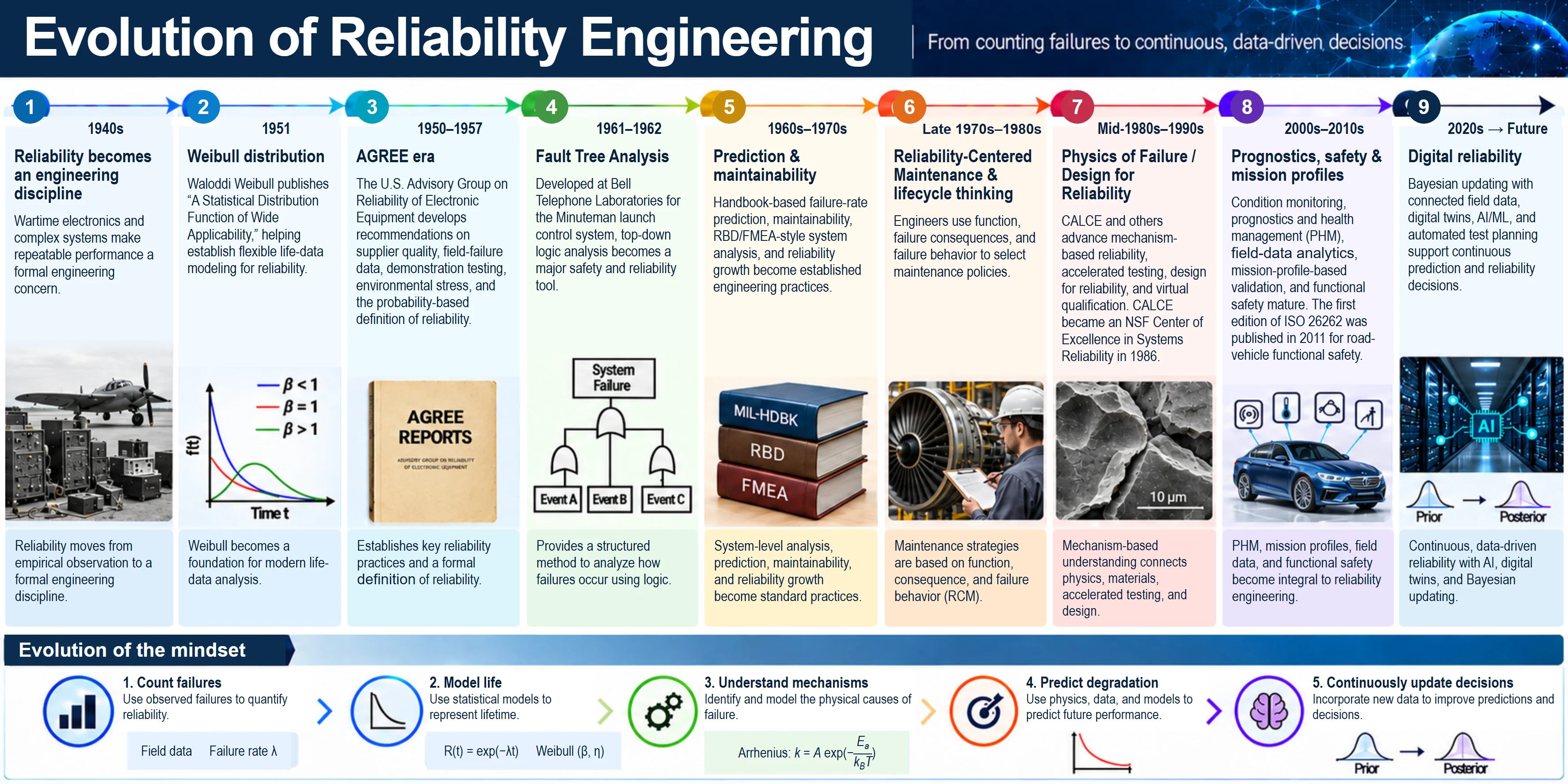
This article walks through the nine eras in the infographic below. For each one it covers what changed, the governing equation, and what it means for your next program. The same 22-unit test returns in Section 3 (AGREE) and Section 9 (Bayesian updating), so you can see how the answer to one question changed over 70 years. Every era links to a free Reliatools calculator, with the exact inputs to reproduce the worked example yourself.
Calculators in this article
| Era | Method | Free Reliatools calculator |
|---|---|---|
| 1940s | Series system reliability (Lusser's law) | Reliability Block Diagram Calculator |
| 1951 | Weibull life data analysis | Weibull Analysis Calculator |
| 1951 | Infant mortality screening (β < 1) | Burn-In Test Planning Wizard |
| 1957 | Demonstration testing | Sample Size Calculator |
| 1962 | Risk of new designs and conditions | NUDD Assessment |
| 1969 | Black's equation | Electromigration MTTF Calculator |
| 1961–1995 | Failure rate budgets | FIT Calculator |
| 1980s–1990s | Temperature acceleration | Arrhenius Acceleration Factor Calculator |
| 1980s–1990s | Thermal-cycling fatigue | Coffin-Manson Thermal Fatigue Calculator |
| 1980s–1990s | Step-stress margin discovery | HALT/HASS Test Plan Builder |
| 1980s–1990s | Robust design | P-Diagram Generator |
| 2000s–2010s | Mission profiles | Mission Profile & Duty Cycle Builder |
| 2000s–2010s | Vibration and humidity conditions | Vibration PSD Profile Builder, Psychrometric Calculator |
| 2000s–2010s | Test planning and margins | Reliability Test Plan Generator, Component Derating Navigator |
| 2020s | Bayesian updating | Bayesian Software Reliability Predictor |
1. 1940s: Reliability becomes an engineering discipline
World War II put complex electronics into the field at scale. Radar, communications and fire-control systems depended on vacuum tubes that failed often and unpredictably. Repeatable failure performance became a formal engineering concern rather than a hope.
The first quantitative insight came from the German V-1 program. Robert Lusser, working with the development team, showed that a system made of parts in series is only as reliable as the product of its part reliabilities.
Worked example. A system of 100 parts, each 99% reliable, has
Two out of three systems fail even though every part looks "good". To reach a system reliability of 0.90, each of the 100 parts needs a reliability of about 0.999.
Physics of failure note. Lusser's law assumes independent failures. Shared stresses such as a hot enclosure or a common supply transient break that assumption, as one stress acts on many parts at once.
2. 1951: Weibull distribution
In 1951 Waloddi Weibull published A Statistical Distribution Function of Wide Applicability in the ASME Journal of Applied Mechanics. Its strength was flexibility, as one shape parameter can describe early failures, random failures or wear-out.
Reading the infographic: Panel 2 plots the probability density f(t), which shows when failures occur. The table below describes the hazard rate h(t), which shows the risk of failure for units still running. For β > 1 the density rises to a peak and then falls, while the hazard keeps rising.
| Shape β | Hazard rate h(t) | Typical physical meaning | Reliatools tool |
|---|---|---|---|
| β < 1 | Decreasing | Infant mortality from manufacturing defects | Burn-In Test Planning Wizard |
| β = 1 | Constant | Random overstress events (exponential case) | FIT Calculator |
| β > 1 | Increasing | Wear-out such as fatigue, corrosion or diffusion | Weibull Analysis Calculator |
Physics of failure note. A fitted β describes how the population hazard changes with age. Use β to guide the failure investigation, and confirm the mechanism through failure analysis.
3. 1950–1957: AGREE era
The U.S. Department of Defense formed an Ad Hoc Group on Reliability of Electronic Equipment in December 1950. In August 1952 it became the permanent Advisory Group on Reliability of Electronic Equipment (AGREE). Its report, issued on June 4, 1957, covered supplier quality, field failure data, environmental stress and demonstration testing.
AGREE's lasting contribution was the probability-based definition that every engineer still uses. Reliability is the probability that an item performs its required function, under stated conditions, for a stated period of time. That definition made reliability something that could be specified, allocated and demonstrated.
Demonstration testing follows directly. With zero failures allowed, the success-run sample size is
Worked example. Demonstrating R = 0.90 at C = 90% needs n = ln(0.10)/ln(0.90) = 21.9, so 22 units with zero failures. Raising the target to R = 0.95 needs 45 units.
What it means today. Every requirement needs all four parts of the AGREE definition: function, conditions, duration and probability. A requirement missing the "stated conditions" part cannot be validated.
4. 1961–1962: Fault Tree Analysis
H. A. Watson at Bell Telephone Laboratories developed fault tree analysis in 1961–62 under a U.S. Air Force contract for the Minuteman I launch control system. FTA works top-down. It starts from one undesired system event and uses AND/OR logic to trace every combination of lower-level events that can cause it.
For independent input events, the gate probabilities are
The independence condition carries the same warning as Lusser's law in Section 1. If both branches of an AND gate depend on the same power supply, model that shared cause explicitly as its own basic event. Otherwise the tree will report a redundant design as far more reliable than it is.
The same year saw a second milestone that is often forgotten. The Rome Air Development Center held the first Physics of Failure in Electronics symposium in Chicago in September 1962. That series became today's International Reliability Physics Symposium (IRPS). Physics of failure is therefore not a modern idea. It is as old as the fault tree.
One of the best-known results from that community is Black's equation for electromigration in metal interconnects, published by J. R. Black in 1969. It ties life directly to current density and temperature.
The negative exponent on J matters, as higher current density shortens life. With n = 2, doubling current density cuts MTTF to one quarter.
5. 1960s–1970s: Prediction & maintainability
The first edition of MIL-HDBK-217, Reliability Prediction of Electronic Equipment, was published in 1961. It built on earlier work such as RCA's TR-1100 and gave each part type a base failure rate multiplied by stress, quality and environment factors.
Handbook prediction made system-level failure budgets possible, as constant rates add for a series system. FMEA, maintainability analysis and reliability block diagrams became standard practice in the same period.
In 1964 J. T. Duane of General Electric published the observation behind reliability growth. On log-log axes, cumulative MTBF rises roughly linearly with cumulative test time when failures are found and fixed.
A growth rate α of 0.3 to 0.5 typically indicates an active test-analyze-fix program. A slope near zero means cumulative MTBF shows little observed improvement. Check whether corrective actions have been implemented and whether enough test exposure has accumulated to see their effect.
Physics of failure note. A constant λ implies β = 1, so it cannot represent wear-out. Handbook predictions are budgets, not life predictions.
6. Late 1970s–1980s: Reliability-Centered Maintenance & lifecycle thinking
Commercial aviation drove the next shift. Airline maintenance steering groups developed decision logic for the Boeing 747 (MSG-1, 1968). In December 1978 F. Stanley Nowlan and Howard Heap of United Airlines published Reliability-Centered Maintenance for the Department of Defense.
Their analysis of airline data showed that many failure patterns do not have a clear wear-out age. For those items, scheduled overhaul at a fixed age does little to reduce failures and can add infant-mortality failures after the work is done. Maintenance should instead follow the function of the item, the consequence of its failure and its actual failure behavior.
What it means today. The same lifecycle logic applies in design. Before you specify a test, ask what failure behavior the mechanism shows and what the consequence of that failure is. A wear-out mechanism justifies a durability test. A random overstress mechanism justifies margin and protection.
7. Mid-1980s–1990s: Physics of Failure / Design for Reliability
In 1985 the U.S. Army asked the University of Maryland to update MIL-HDBK-217. The researchers concluded that the statistical approach behind the handbook could not predict the reliability of new technologies or guide design. That work founded CALCE, which became a National Science Foundation Center of Excellence in Systems Reliability in 1986.
The physics-of-failure approach models each mechanism directly from stress, material and geometry. Two models carry most of the load in electronics.
Arrhenius (temperature-driven mechanisms)
The infographic shows Arrhenius in its rate form, k = A exp(−Eₐ / k_B T). The acceleration factor is the ratio of the rates at the stress and use temperatures, so the constant A cancels.
Worked example. With Eₐ = 0.7 eV, T_use = 55 °C (328.15 K) and T_stress = 125 °C (398.15 K), AF = 77.6. One hour at 125 °C represents about 78 hours at 55 °C for that mechanism only.
Coffin-Manson (thermal-cycling fatigue)
The simplified temperature-range form of the model relates cycles to failure at two temperature swings.
Worked example. Cycling from −40 °C to 125 °C (ΔT = 165 °C) against a field ΔT of 60 °C with n = 2 gives a ratio of (165/60)² = 7.6. For the assumed exponent and the same fatigue mechanism, the model predicts about 7.6 field cycles per test cycle.
Three events in this period turned physics of failure into practice.
| Year | Event | Effect | Reliatools tool |
|---|---|---|---|
| Late 1980s | HALT and HASS developed by Gregg Hobbs | Step-stress testing to find design margins and operating limits | HALT/HASS Test Plan Builder |
| June 29, 1994 | Perry memo on military specifications | DoD gave preference to commercial and performance standards over MIL-STDs | — |
| 1994 | AEC-Q100 issued by the Automotive Electronics Council (Chrysler, Ford, GM) | Failure-mechanism-based stress qualification for automotive ICs | Reliability Test Plan Generator |
MIL-HDBK-217 received its final update, Revision F Notice 2, on February 28, 1995.
Robust design also spread through US industry in this period. Taguchi's methods framed reliability as performance that stays on target despite noise factors such as temperature, humidity, vibration and part-to-part variation.
8. 2000s–2010s: Prognostics, safety & mission profiles
Automotive electronics moved from qualify-to-a-list to qualify-to-the-application. In April 2007 ZVEI published the Handbook for Robustness Validation of Semiconductor Devices in Automotive Applications, with SAE adopting it as J1879 in October 2007. Its core principle is to design in sufficient margin between the loads of the mission profile and the real capability of the component.
ISO 26262 published its first edition in 2011 for road-vehicle functional safety, with a second edition in 2018. Reliability data now fed safety metrics such as the probabilistic metric for random hardware failures (PMHF).
In parallel, condition monitoring and prognostics and health management (PHM) used sensor and field data to estimate the remaining useful life of individual units rather than of populations.
What it means today. Start every validation plan from a mission profile, not from a standard's test list.
9. 2020s → Future: Digital reliability
The newest layer does not replace the older ones. It connects them. Connected products return field data continuously, digital twins carry physics-of-failure models through the product's life, and Bayesian updating combines prior knowledge with new evidence. AI/ML models and automated test planning draw on the same data, so prediction and decisions can be updated as evidence arrives rather than once per program.
Bayesian methods have existed in reliability for decades. What changed is the volume of data that now feeds them. The Beta-Binomial model shows the idea for a pass/fail test.
Worked example. Return to the 22 units from Section 3, all passing with zero failures.
| Approach | Calculation | 90% lower bound on R |
|---|---|---|
| Classical (exact one-sided confidence bound) | 0.9006 | |
| Bayesian, uniform prior Beta(1, 1) → posterior Beta(23, 1) | 0.9047 | |
| Bayesian, prior from previous generation worth 9 extra passes → posterior Beta(32, 1) | 0.931 |
Both of the first two approaches put the lower bound just above 90%. The Bayesian result also reflects the chosen prior. An informative prior from a previous generation raises the bound to 0.931 with the same 22 units.
Physics of failure note. The prior is only valid when the earlier data came from comparable failure mechanisms under comparable stress conditions. A prior from a different material set, process or mission profile can make a weak design look demonstrated. Check this assumption before taking any test credit.
What it means today. Treat test data as a long-term asset. Store it with its conditions, failure modes and mechanisms so that the next program can use it as a defensible prior.
Evolution of the mindset
Each era added a question rather than replacing the last one.
| Stage | Question asked | Typical method | Governing form | Run it in Reliatools |
|---|---|---|---|---|
| 1. Count failures | How often does it fail? | Field data, failure rate λ | λ = failures / unit-hours | FIT Calculator |
| 2. Model life | How is life distributed? | Exponential, Weibull (β, η) | R(t) = exp(−λt), R(t) = exp[−(t/η)^β] | Weibull Analysis Calculator |
| 3. Understand mechanisms | Why does it fail? | Physics of failure, accelerated testing | Arrhenius k = A exp(−Eₐ / k_B T) | Arrhenius, Coffin-Manson |
| 4. Predict degradation | When will this unit fail in this use? | Physics, data and models applied to the mission profile | Damage accumulation against the mission profile | Mission Profile & Duty Cycle Builder |
| 5. Continuously update decisions | What does new evidence change? | Bayesian updating, digital twins | Prior → posterior | Bayesian Software Reliability Predictor |
What this means for your next program
- Start with the mission profile. Every later step depends on stated conditions, which has been true since AGREE in 1957.
- Name the mechanism before choosing the model. Arrhenius for temperature-driven chemistry, Coffin-Manson for thermal fatigue, Black's equation for electromigration, and a separate acceleration factor for each.
- Use handbook failure rates for budgets only. They assume β = 1 and say nothing about wear-out life.
- Keep your test data. Data stored with its conditions and mechanisms becomes the prior that shortens the next program.
The first step is the one most programs skip. Build your mission profile in the Mission Profile & Duty Cycle Builder.
Timeline reference: key dates and sources
| Date | Milestone |
|---|---|
| 1940s | Lusser's product law from the V-1 program; wartime vacuum-tube failures |
| Dec 1950 / Aug 1952 | DoD Ad Hoc Group on Reliability, then AGREE |
| 1951 | Weibull publishes A Statistical Distribution Function of Wide Applicability |
| June 4, 1957 | AGREE report published |
| 1961 | MIL-HDBK-217 first edition |
| 1961–1962 | Fault tree analysis at Bell Labs for Minuteman I |
| Sept 1962 | First Physics of Failure in Electronics symposium (RADC) |
| 1964 | Duane reliability growth model |
| 1968 | MSG-1 maintenance logic for the Boeing 747 |
| 1969 | Black's equation for electromigration |
| Dec 1978 | Nowlan and Heap, Reliability-Centered Maintenance |
| 1985 / 1986 | CALCE founded; becomes an NSF Center of Excellence |
| Late 1980s | HALT/HASS developed |
| June 1994 | Perry memo on military specifications and standards |
| 1994 | AEC-Q100 issued |
| Feb 1995 | MIL-HDBK-217F Notice 2, the final revision |
| 2007 | Robustness Validation handbook (ZVEI, SAE J1879) |
| 2011 / 2018 | ISO 26262 first and second editions |
| 2020s | Connected field data, digital twins, AI/ML, Bayesian updating at scale |
References
- Weibull, W. (1951). A Statistical Distribution Function of Wide Applicability. Journal of Applied Mechanics, 18, 293–297.
- Advisory Group on Reliability of Electronic Equipment (1957). Reliability of Military Electronic Equipment. Office of the Assistant Secretary of Defense (R&E).
- Bell Telephone Laboratories (September 15, 1962). Launch Control Safety Study (H. A. Watson). Prepared for the U.S. Air Force, Minuteman I.
- Rome Air Development Center (1962). Physics of Failure in Electronics, First Annual Symposium, Chicago.
- Duane, J. T. (1964). Learning Curve Approach to Reliability Monitoring. IEEE Transactions on Aerospace, 2(2).
- Black, J. R. (1969). Electromigration: A Brief Survey and Some Recent Results. IEEE Transactions on Electron Devices, 16(4), 338–347.
- Nowlan, F. S. and Heap, H. F. (1978). Reliability-Centered Maintenance. United Airlines for the U.S. Department of Defense.
- U.S. Department of Defense (1995). MIL-HDBK-217F Notice 2, Reliability Prediction of Electronic Equipment.
- Secretary of Defense (June 29, 1994). Memorandum, Specifications and Standards: A New Way of Doing Business.
- Automotive Electronics Council. AEC-Q100, Failure Mechanism Based Stress Test Qualification for Integrated Circuits.
- ZVEI / SAE (2007). Handbook for Robustness Validation of Semiconductor Devices in Automotive Applications (SAE J1879).
- ISO 26262 (2011, 2018). Road vehicles: Functional safety.
- National Research Council (2015). Reliability Growth: Enhancing Defense System Reliability, Appendix D: Critique of MIL-HDBK-217. National Academies Press.
- NIST/SEMATECH. e-Handbook of Statistical Methods, Section 8.1.6.2, Weibull.
Related calculators
- Weibull Probability Plot
Fit 2-parameter Weibull to failure and suspension data; get beta, eta and B-lives.
- Sample Size Calculator
Size a test by what it must prove: success run, MTBF, Weibayes, A/B and more.
- Arrhenius Calculator
Acceleration factors, equivalent life and test durations for temperature-driven aging.